K-Nearest Neighbors Algorithm using Python and Scikit-Learn

K nearest Neighbors (kNN) works based on calculating distance between given test data point and all the training samples. We, then, collect first K closest points from training set and the majority vote gives you the predicted class for a given test data point.

For more intuitive explanation, please follow previous post :

How kNN works ?

In [1]:
import math
from collections import Counter
import numpy as np
import pandas as pd
import matplotlib.pyplot as plt

%matplotlib inline

# making results reproducible
np.random.seed(42)
In [2]:
df = pd.read_csv(
    'https://archive.ics.uci.edu/ml/machine-learning-databases/wine/wine.data', header=None, sep=',')

df.columns = ['CLASS', 'ALCOHOL_LEVEL', 'MALIC_ACID', 'ASH', 'ALCALINITY','MAGNESIUM', 'PHENOLS', 
              'FLAVANOIDS', 'NON_FLAVANOID_PHENOL', 'PROANTHOCYANINS', 'COLOR_INTENSITY', 
              'HUE', 'OD280/OD315_DILUTED','PROLINE']

# Let us use only two features : 'ALCOHOL_LEVEL', 'MALIC_ACID' for this problem
df = df[['CLASS', 'ALCOHOL_LEVEL', 'MALIC_ACID']]
df.head()
Out[2]:
CLASS ALCOHOL_LEVEL MALIC_ACID
0 1 14.23 1.71
1 1 13.20 1.78
2 1 13.16 2.36
3 1 14.37 1.95
4 1 13.24 2.59
In [3]:
# class distribution looks okay; not so imbalanced.
df['CLASS'].value_counts().plot(kind="bar")
plt.show()
No description has been provided for this image

How do I know Principal Component Analysis (PCA) is preserving information from my data ?

Principal Component Analysis is used for dimension reduction of high-dimensional data. We also refer PCA as feature extraction technique, where new features take the linear combinations from original features.

More on PCA : principal-component-analysis-pca-for-visualization-using-python

In this post, we will investigate 'how reliable the information is as preserved by PCA'. In order to do that, we will use labelled data and evaluate the trained model to see the final performance. (In side note, PCA is unsupervised learning algorithm. But, in our case, we are using in supervised fashion to assess the model performance)

To make it more interesting, we will also see Random Forests as 'feature selection' and compare the result with PCA.

1. PCA as Feature Extraction

In [13]:
%matplotlib inline

import numpy as np
import seaborn as sns
import matplotlib.pyplot as plt
import pandas as pd 

from sklearn.preprocessing import StandardScaler
from sklearn.model_selection import train_test_split
from sklearn.metrics import accuracy_score
from sklearn.ensemble import RandomForestClassifier
from sklearn.tree import DecisionTreeClassifier
In [14]:
df = pd.read_csv(
    'https://archive.ics.uci.edu/ml/machine-learning-databases/wine/wine.data', header=None, sep=',')

df.columns = ['CLASS', 'ALCOHOL_LEVEL', 'MALIC_ACID', 'ASH', 'ALCALINITY','MAGNESIUM', 'PHENOLS', 
              'FLAVANOIDS', 'NON_FLAVANOID_PHENOL', 'PROANTHOCYANINS', 'COLOR_INTENSITY', 
              'HUE', 'OD280/OD315_DILUTED','PROLINE']
df.head()
Out[14]:
CLASS ALCOHOL_LEVEL MALIC_ACID ASH ALCALINITY MAGNESIUM PHENOLS FLAVANOIDS NON_FLAVANOID_PHENOL PROANTHOCYANINS COLOR_INTENSITY HUE OD280/OD315_DILUTED PROLINE
0 1 14.23 1.71 2.43 15.6 127 2.80 3.06 0.28 2.29 5.64 1.04 3.92 1065
1 1 13.20 1.78 2.14 11.2 100 2.65 2.76 0.26 1.28 4.38 1.05 3.40 1050
2 1 13.16 2.36 2.67 18.6 101 2.80 3.24 0.30 2.81 5.68 1.03 3.17 1185
3 1 14.37 1.95 2.50 16.8 113 3.85 3.49 0.24 2.18 7.80 0.86 3.45 1480
4 1 13.24 2.59 2.87 21.0 118 2.80 2.69 0.39 1.82 4.32 1.04 2.93 735
In [15]:
features = ['ALCOHOL_LEVEL', 'MALIC_ACID', 'ASH', 'ALCALINITY','MAGNESIUM', 'PHENOLS', 
              'FLAVANOIDS', 'NON_FLAVANOID_PHENOL', 'PROANTHOCYANINS', 'COLOR_INTENSITY', 
              'HUE', 'OD280/OD315_DILUTED','PROLINE']
label = 'CLASS'

X = df[features]
y = df[label]

# train test split with 70% for training
X_train, X_test, y_train, y_test = train_test_split(X, y, test_size=0.3, random_state=0)
a. Preparing Projected data using PCA
In [16]:
# prepare correlation matrix
# standar scaler for normalization
N, _ = df.shape
scaler = StandardScaler()
Z = scaler.fit_transform(X)
# Correlation estimation
R = np.dot(Z.T, Z) / N

# eigendecomposition
eigen_values, eigen_vectors = np.linalg.eig(R)

# prepare projection matrix
value_idx = eigen_values.argsort()[::-1]
eigen_vectors_sorted = eigen_vectors[:, value_idx]

# Projection matrix with 3 PCs ( 3 PCs cover 65% variance in the data)
# more on : https://sijanb.com.np/posts/principal-component-analysis-pca-for-visualization-using-python/
M = np.hstack((eigen_vectors_sorted[0][:, np.newaxis],
               eigen_vectors_sorted[1][:, np.newaxis],
               eigen_vectors_sorted[2][:, np.newaxis]))

# projected data
projected_data = np.asmatrix(Z) * np.asmatrix(M)
b. Using Projected data for the training and prediction using Decision Tree
In [17]:
# train test split for training
Xpc_train, Xpc_test, ypc_train, ypc_test = train_test_split( projected_data, y, test_size=0.3, random_state=0)

tree_pca = DecisionTreeClassifier(max_depth=6, random_state=0)
tree_pca.fit(Xpc_train, ypc_train)

ypca_pred = tree_pca.predict(Xpc_test)
print('Test accuracy using Decision tree on PCA projected data: %.2f' % accuracy_score(ypc_test, ypca_pred))
Test accuracy using Decision tree on PCA projected data: 0.76

Principal Component Analysis (PCA) for Visualization using Python

1. Basic Setup

Principal Component Analysis (PCA) is being used to reduce the dimensionality of data whilst retaining as much of information as possible. The general idea of PCA works as follows:

 a. Find the principal components from your original data
 b. Project your original data into the space spanned by principal components from (a)

Let's use $ \textbf{X} $ as our data matrix and $ \sum $ as our covariance matrix of $ \textbf{X} $. We will get eigenvectors ( $ \bf{v_1}, {v_2}, .....{v_k} $) and eigenvalues (${\lambda_1},{\lambda_2},....,{\lambda_k}$) from the covariance matrix $ \sum $, such that:

$ \lambda_1 \geq \lambda_2 \geq ...... \lambda_k $

NOTE* : Elements of the vector ($ \bf{v_1} $ ) represents the coefficients of principal components.

Our goal is to maximize the variance of projection along each of principal components. This can be written as:

$ \bf{var(y_i)} = \bf{var}(v_{i1} * X_1 + v_{i2} * X_2 + ...... + v_{ik} * X_k ) $

You can see that, we are projecting the original data into our new vector space given by PCs.

NOTE* : $ \bf{var(y_i)} = \lambda_i $ and principal components are uncorrelated i.e $ cov(y_i, y_j) $ = 0

2. Principal Component Analysis Algorithm (Pseudocode)

a. $ \textbf{X} \gets $ design data matrix with dimension ( N*k )

b. $ \textbf{X} \gets $ subtract mean from each column vector of $ \bf{X} $

c. $ \sum \gets $ compute covariance matrix of $ \bf{X} $

d. Calculate eigenvectors and eigenvalues from $ \sum $

e. Principal Components (PCs) $ \gets $ the first M eigenvectors with largest eigenvalues.

3. Basic Data Analysis

Sijan Bhandari on

Linear Regression with Maximum Likelihood (MSE) and Bayesian Learning Approach from scratch

1. Setup

Given the input dataset $ \textbf{D} = \{(x_i, t_i)\}_{i=1}^{N} $, our goal is to learn the parameters that model this data and use those parameters (w) for the prediction new data point.

We often define the features (basis functions) as : $ \{ \phi_1(x),......,\phi_m(x) \} $ and the linear regression model is defined as :

$ y(x,w) = \sum_{i=1}^m w_i \phi_i (x) + \varepsilon_i $

$ \varepsilon_i $ suggesting that we can not perfectly model the data generation process and there will be certain noise in our designed model(paramters). Usually, we assume that the noise is Gaussian. $ \varepsilon_i \sim Normal(0, \beta^{-1} )$

2. Objective Functions

a. Maximum Likelihood objective (MLE) .i.e . ( Mean Squared Error )

J(w) = $ \frac{1}{2} \sum_i^N \{t_i - w^T \phi(x_i) \}^2 $

b. Regularized Linear Regression

J(w) = $ \frac{1}{2} \sum_i^N \{t_i - w^T \phi(x_i) \}^2 $ + $ \frac{\lambda}{2} w^T w $

3. Closed Form Solutions

a. For MSE

$ w_{MLE} = ( \phi^T \phi )^{-1} \phi^T t $

$ ( \phi^T \phi )^{-1} $ is called Moore-Penrose inverse.

b. For Regularized MSE

$ w_{MLE} = ( \lambda I + \phi^T \phi )^{-1} \phi^T t $

4. Bayesian Learning

By using Bayes rule, we have :

$ p(w | t) = \frac{p(t|w)p(w)}{p(t)} $

$ p(w|t) $ - Posterior distribution $ p(t|w) $ - Likelihood of data given parameters $ p(w) $ - Prior distribution over paramters (w)

a. Pior on w :

Understanding Regularization for Support Vector Machines (SVMs)

I would like you to go through Intuition Behind SVM before exploring about Regularization.

SVM has an objective To find the optimal linearly speparating hyperplane which maximizes the margin. But, we know that Hard-Margin SVM can work well when data is completely lineary separable (without any noise or outliers). What if our data is not perfectly separable? We have two options for non-separable data:

 a. Using Hard-Margin SVM with feature transformations
 b. Using Soft-Margin SVM

If you want a good generalization on your result, we should tolerate some errors. If we force our model to be perfect, it will be just an attempt to overfit the data!.

Let's talk about Soft-Margin SVM and it helps us to understand Regularization. If the training data is not linearly separable, we allow our hyperplane to make few mistakes on outliers or say noisy data. Mistakes means those outliers/noise data can be inside the margin or on the wrong side of the margin.

But, we will have a mechanism to pay a cost for each of those misclassified example. That cost will depend on how far the data point is from the margin. This cost is represented by slack variables ($ξ_i$)

objective function : $ \frac{1}{2} ||w||^2 + C \sum_{i=1}^{n} ξ_i $

In the above equation, the parameter C defines the strength of regularization. We can discuss three different cases based on values of C:

Sijan Bhandari on

Implementation of K means clustering algorithm in Python

For K means clustering algorithm, I will be using Credit Cards Dataset for Clustering from Kaggle.

In [135]:
import numpy as np
import pandas as pd

import matplotlib.pyplot as plt

%matplotlib inline

Data preprocessing

In [136]:
credit_data = pd.read_csv('../data/CC GENERAL.csv')
In [137]:
credit_data.head()
Out[137]:
CUST_ID BALANCE BALANCE_FREQUENCY PURCHASES ONEOFF_PURCHASES INSTALLMENTS_PURCHASES CASH_ADVANCE PURCHASES_FREQUENCY ONEOFF_PURCHASES_FREQUENCY PURCHASES_INSTALLMENTS_FREQUENCY CASH_ADVANCE_FREQUENCY CASH_ADVANCE_TRX PURCHASES_TRX CREDIT_LIMIT PAYMENTS MINIMUM_PAYMENTS PRC_FULL_PAYMENT TENURE
0 C10001 40.900749 0.818182 95.40 0.00 95.4 0.000000 0.166667 0.000000 0.083333 0.000000 0 2 1000.0 201.802084 139.509787 0.000000 12
1 C10002 3202.467416 0.909091 0.00 0.00 0.0 6442.945483 0.000000 0.000000 0.000000 0.250000 4 0 7000.0 4103.032597 1072.340217 0.222222 12
2 C10003 2495.148862 1.000000 773.17 773.17 0.0 0.000000 1.000000 1.000000 0.000000 0.000000 0 12 7500.0 622.066742 627.284787 0.000000 12
3 C10004 1666.670542 0.636364 1499.00 1499.00 0.0 205.788017 0.083333 0.083333 0.000000 0.083333 1 1 7500.0 0.000000 NaN 0.000000 12
4 C10005 817.714335 1.000000 16.00 16.00 0.0 0.000000 0.083333 0.083333 0.000000 0.000000 0 1 1200.0 678.334763 244.791237 0.000000 12
A. Check for missing data
In [138]:
credit_data.isna().sum()
Out[138]:
CUST_ID                               0
BALANCE                               0
BALANCE_FREQUENCY                     0
PURCHASES                             0
ONEOFF_PURCHASES                      0
INSTALLMENTS_PURCHASES                0
CASH_ADVANCE                          0
PURCHASES_FREQUENCY                   0
ONEOFF_PURCHASES_FREQUENCY            0
PURCHASES_INSTALLMENTS_FREQUENCY      0
CASH_ADVANCE_FREQUENCY                0
CASH_ADVANCE_TRX                      0
PURCHASES_TRX                         0
CREDIT_LIMIT                          1
PAYMENTS                              0
MINIMUM_PAYMENTS                    313
PRC_FULL_PAYMENT                      0
TENURE                                0
dtype: int64

We can see that some missing values in column MINIMUM_PAYMENTS column. Since we are focusing on algorithm aspect in this tutorial, I will simply remove entries having 'NaN' value.

B. Remove 'NaN' entries
In [139]:
credit_data = credit_data.dropna(how='any')
C. Remove nonrelevant column/feature
In [140]:
# Customer ID does not bear any meaning to build cluster. So, let's remove it.
credit_data.drop("CUST_ID", axis=1, inplace=True)
Sijan Bhandari on

Intuition behind Gradient Descent for Machine Learning Algorithms

No description has been provided for this image

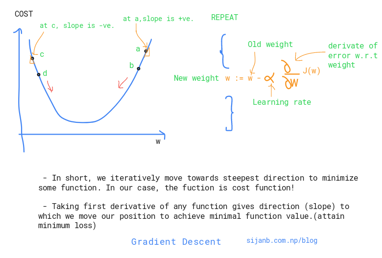
Before jumping to Gradient Descent, let's be clear about difference between backpropagation and gradient descent. Comparing things make it easier to learn !

Backpropagation :

Backpropagation is an efficient way of calculating gradients using chain rule.

Gradient Descent:

Gradient Descent is an optimization algorithm which is used in different machine learning algorithms to find parameters/combination of parameters which mimimizes the loss function.

** In case of neural network, we use backpropagation to calculate the gradient of loss function w.r.t to weights. Weights are the parameters of neural network.

** In case of linear regression, coefficients are the parameters!.

** Many machine learning algorithms are convex problems, so using gradient descent to get extrema makes more sense. For example, if you remember the solution of linear regression :

$ \beta = (X^T X)^{-1} X^T y $

Here, we can get the analytical solution by simply solving above equations. But, inverse calculation has $ O(N^3) $ complexity. It will be worst if our data size increases.

Sijan Bhandari on

Interpreting Centrality Measures for Network Analysis

Network has been taken as a tool for describing complex systems or interactions around us. Few prominent complex systems are:

  1. Our society where almost 7 billions individuals exist/ and the interactions between them in one or other ways.

  2. Genes in our body, interactions between gene molecules ( Protein-Protein interaction networks)

Peoply usually visualize the network to see cluter/ densely linked clusters and try to analyze, predict relation between nodes, figure out similarity between nodes in the network.

Figuring out the central nodes/vertices is also an important network analysis process because centrality measures :

        a. Existing influence of a node on other nodes
        b. Information flow in and out from a node or towards it
        c. Finding node/s which is/are acting as bridge between two different/big groups
Sijan Bhandari on

Understanding Term Frequencey and Inverse Document Frequency

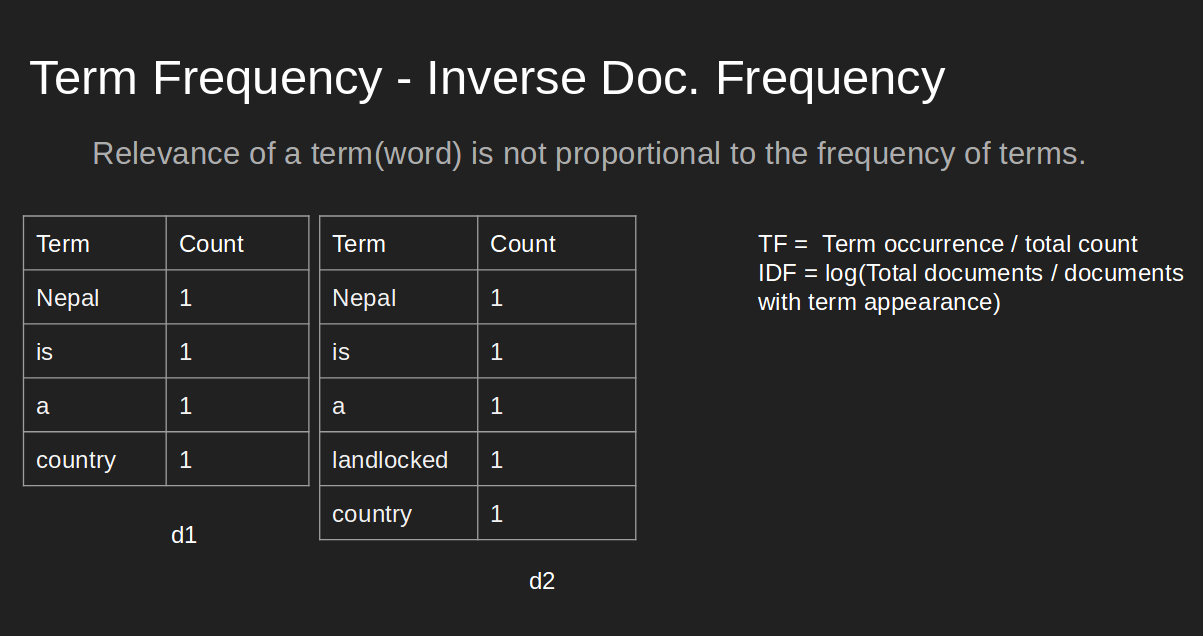
In any document, the frequency of occurrence of terms is taken as an important measure of score for that document (Term Frequency). For example : a document has total 100 words, and 30 words are 'mountains', we ,without hesitation, say that this document is talking about 'Mountains'.

But, if we only include most frequent word as our score metric, we will eventually loose the actual relevancy score of the document. Since same word could exist in number of documents and it's just frequent occurrence without adding much meaning to current context. In the above example : Suppose, there are two documents talking about 'Mt. Everest'. We obviously know that there will be higher occurrence of word 'Mountains'. But, if we use 'Term Frequecy (tf)' alone, term 'Mountains' will get highest weight rather than term 'Everest'. It's not fair. And, Inverse-Document-Frequency will tackle it.

Term Frequency (TF) / Normalized Term Frequency (nTF):

It simply measures the frequency/occurent of a term in a document. So, it gives equal important to all terms. Longer document could have large number of terms than smaller documents, so better to normalize this metric by dividing with total number of terms in the document. We also

Applications:

  1. Summarizing a document by extracting keywords.
  2. Comparing two documents (similary/ relevancy check)
  3. Search query to documents matching for building query results for search engine
  4. Weighting 'terms' in the document.

Inverse Document Frequency (IDF):

It gives the importance to more relevant/significant term in the document. It tries to lower the weights to terms having less importance. And, rare terms will get significant weights.

TF-IDF:

It tries to prioritize the terms based on their occurrence and uniqueness.

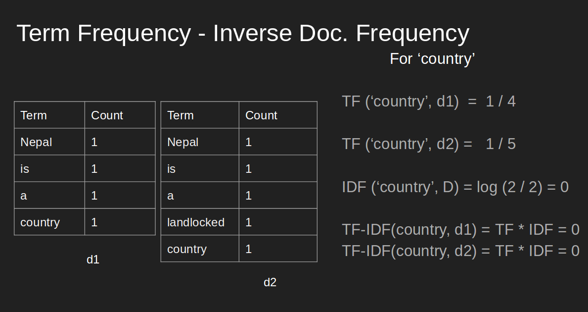
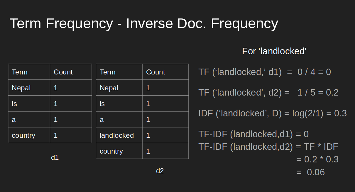
Suppose, I have two documents in my corpus and I want to give tf-idf weighting to the terms.

Document I : 'Nepal is a Country'
Document II : 'Nepal is a landlocked Country'
No description has been provided for this imageNo description has been provided for this imageNo description has been provided for this image

We can see that, although, term 'country' has prominent occurrence, 'tf-idf' gives priority to word 'landlocked' and it carries more information about the document.

NOTE 1 :

These weights are eventually used for vector-space model, where each term represents the axes, and document are the vectors on that space. Since 'tf-idf' value is zero (as shown above)' this representation is very sparse.

NOTE 2 :

Suppose, we are building a search engine system. The query is also converted into vector in vector-space model and compare with documents (NOTE 1) to get the similarity between them.

In [ ]:
 
Sijan Bhandari on