Implementation of stochastic subgradient descent for support vector machine using Python

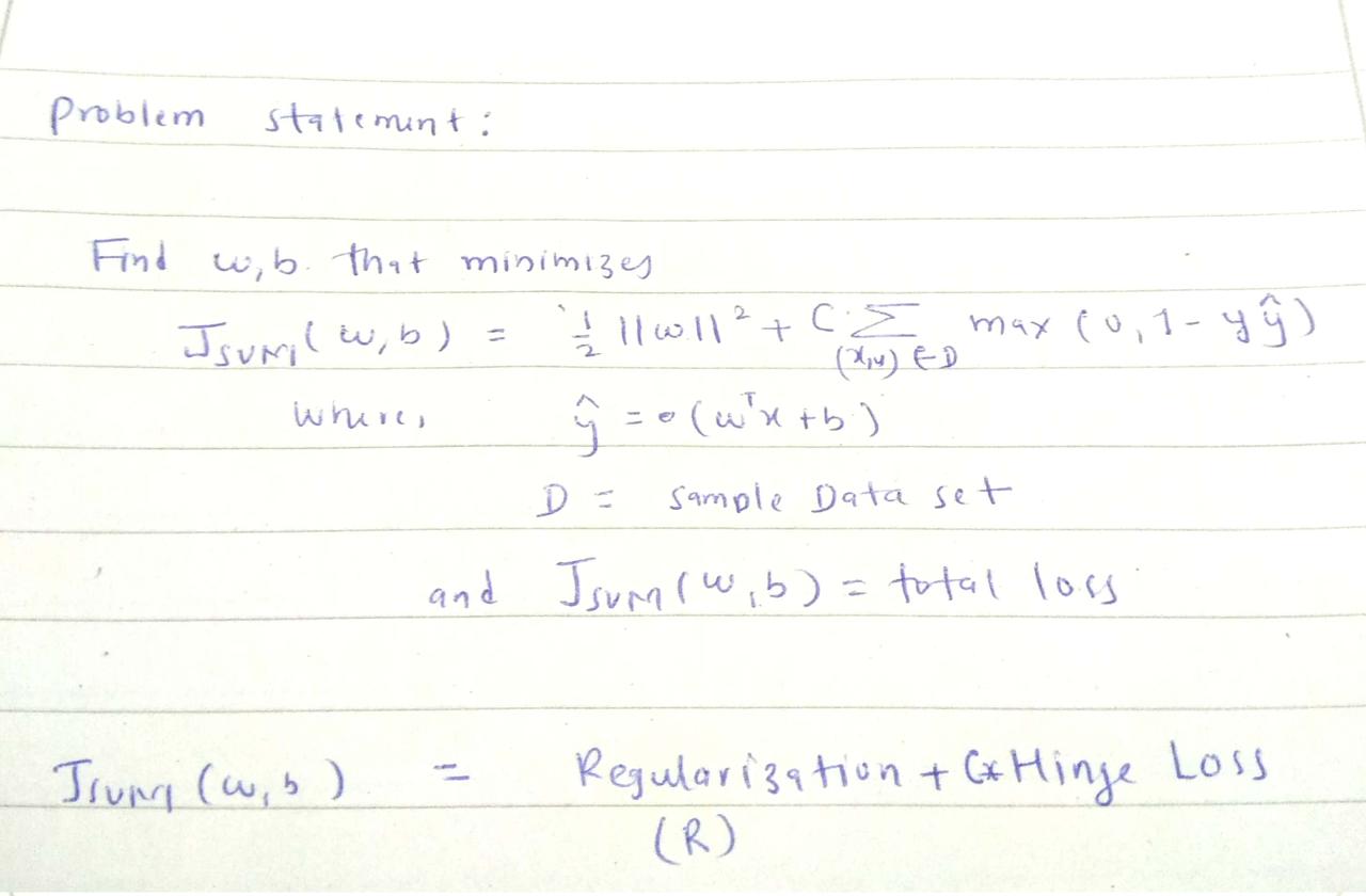
In this post, we will see how we can train support vector machines using stochastic gradient descent (SGD). Before jumping to the algorithm, we need to know why subgradients?

Here is a brief summary of the 0-1 loss and hinge loss:

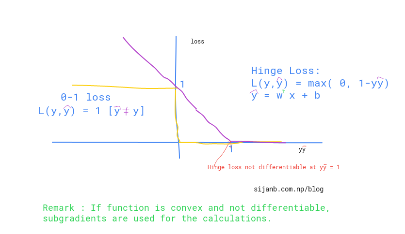
But, why don't we use 0-1 loss ?? The obvious reason is it is not convex. Another factor could be it's reaction to small changes in parameters. You can see from the graph, if you change (w,b) the loss will flip to either 0 or 1 very fast without acknowledging the in between values. The hinge loss,on the other hand, has smooth change until it reaches '1' along x-axis.

In [5]:
import pandas as pd
import numpy as np
In [12]:
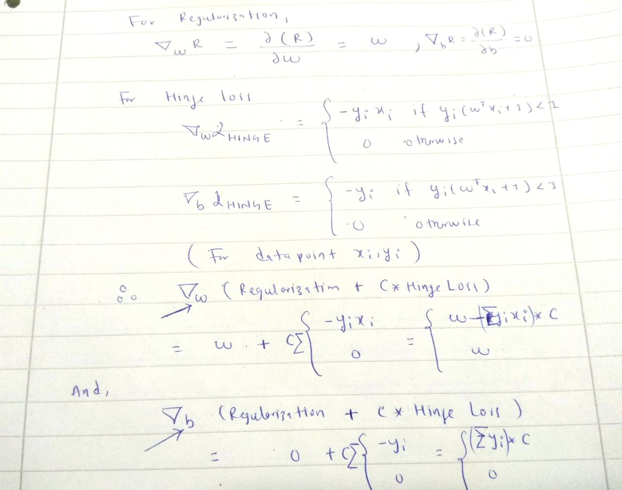
def add_regularization(w, subgradient_w):
    """
    The total loss :( 1/2 * ||w||^2 + Hingle_loss) has w term to be added after getting subgradient of 'w'
    
      total_w = regularization_term + subgradient_term
    i.e total_w = w + C *  ∑ (-y*x)
    
    """
    return w + subgradient_w
In [48]:
def subgradients(x, y, w, b, C):
    """
    :x: inputs [[x1,x2], [x2,x2],...]
    :y: labels [1, -1,...]
    :w: initial w
    :b: initial b
    :C: tradeoff/ hyperparameter
    
    """
    subgrad_w = 0
    subgrad_b = 0
    
    # sum over all subgradients of hinge loss for a given samples x,y
    for x_i, y_i in zip(x,y):
        f_xi = np.dot(w.T, x_i) + b

        decision_value = y_i * f_xi

        if decision_value < 1:
            subgrad_w += - y_i*x_i
            subgrad_b += -1 * y_i
        else:
            subgrad_w += 0
            subgrad_b += 0
    
    # multiply by C after summation of all subgradients for a given samples of x,y
    subgrad_w = C * subgrad_w
    subgrad_b = C * subgrad_b
    return (add_regularization(w, subgrad_w), subgrad_b)
In [49]:
def stochastic_subgrad_descent(data, initial_values, B, C, T=1):
    """
    :data: Pandas data frame
    :initial_values: initialization for w and b
    :B: sample size for random data selection
    :C: hyperparameter, tradeoff between hard margin and hinge loss
    :T: # of iterations
    
    """
    w, b = initial_values
    for t in range(1, T+1):
        
        # randomly select B data points 
        training_sample = data.sample(B)
        
        # set learning rate
        learning_rate = 1/t
        
        # prepare inputs in the form [[h1, w1], [h2, w2], ....]
        x = training_sample[['height', 'weight']].values
      
        # prepare labels in the form [1, -1, 1, 1, - 1 ......]
        y = training_sample['gender'].values
      
        sub_grads = subgradients(x,y, w, b, C)
        
        # update weights
        w = w - learning_rate * sub_grads[0]
        
        # update bias
        b = b - learning_rate * sub_grads[1]
    return (w,b)
In [50]:
data = pd.DataFrame()

data['height'] = np.random.randint(160, 190, 100)
data['weight'] = np.random.randint(50, 90, 100)

data['gender'] = [-1 if value < 5 else 1 for value in np.random.randint(0,10, 100)]

data.head()
Out[50]:
height weight gender
0 167 82 1
1 183 57 -1
2 184 50 -1
3 178 53 -1
4 166 72 1
In [51]:
initial_weights = np.array([-2, -3])
initial_bias = 12

initial_values = (initial_weights, initial_bias)
In [52]:
w,b = stochastic_subgrad_descent(data, initial_values, 20, 1, 1000)
In [53]:
w,b
Out[53]:
(array([-0.798,  4.648]), 14.891692339980313)
In [ ]:
 
Sijan Bhandari on

Why we need Support Vector Machine (SVM) ?

Support vector machine (SVM) is a supervised machine learning algorithm which is considered effective tool for both classification and regression problem.

In a simple word, SVM tries to find a linearly separable hyperplane in order to separate members of one class from another. If SVM can not find the hyperplane for a given data set, it applies non-linear mapping to the training data and transform them to higher dimension where it searches for the optimal hyperplane. The SVM algorithm uses support vectors and margins in order to draw these hyperplanes in the training data.

Since it has ability to understand the complex relation in input data by applying nonlinear mapping, it has high accuracy compare to other supervised classification algorithms (kNN, NCC..)

People have been using SVM for different applications like : text data classification, image data(handwritten) recognition and more.

Intuition:

Let us see a linearly separable problem as shown in the diagram below.

In the given diagram, we can draw infinite lines that can separate data into two different classes.

Can you decide Which of the lines (pink, yellow, green) better suits our problem? If you look closely, the green line is close to red dots and any minor change in data point may caues this point to fall into other class. On the other hand, Pink line is close to blue dots and similarly, a minor twist on data are prone to change the class of new point to other side and may misclassified.

But, the yellow line looks more stable, in the sense, it is far from data points on either side and not susceptible to the small changes in data observations.

Support vector machines help us to make a decision on this problem. If you think 'yellow' line in the figure is the optimal hyperplane for this problem, we can take this as an intuition that an optimal choice from the number of choices of hyperplanes is the one which is farthest from our training data points.

We can compute the perpendicular distances from all our training points to all possible hyperplanes and choose the one which has largest minimum distance to the training examples. The minimum distance between hyperplane and the observation point is called margin.

In summary, SVMs maximize the margin around our separating hyperplane. And, The idea is to draw a margin of some width around the separating hyperplane, up to the nearest point.

The training data that falls exactly on the boundaries of the margin are called

the support vectors. If these points shifted on any direction, they also influence the hyperplanes passing through the margin points and they also shifted. It is important to notice that support vectors are critical data points on our training set since they are the one defining margin boundaries.

It is important to note that the complexity of SVM is characterized by the number of support vectors, rather than the dimension of the feature space. That is the reason SVM has a comparatively less tendency to overfit.

Support vectors "support the plane" and are hence called Support Vectors.

Upto now, we are trying to find the hard-margin for our hyperplane. But, as shown in the diagram below, a single point can have high influence on our boundary. So hard margin SVM are sensitive to outliers, giving overfitted model.

What about we relax our hard margin condition? where, a small amount of data points are allowed to cross the margins/boundaries .i.e data points can be on incorrect side as well. This approach is called soft-margin. Soft in the sense that few data points can violate the margin condition. The softness is measured by slack variable; which control the position of training data points relative to the margins and our hyperplane. The ultimate goal is, our SVM tries to maximize the soft margin.

In [ ]:
 
Sijan Bhandari on

How Nearest Centroid Classifier works?

The Nearest centroid classifier (NCC) says that we should classify a data point to a class whose centroid is closest to this data point.

The algorithms follows:

Suppose $ c_l $ represents the set of indices which belong to class l. And n = |$c_l$|

1.Training step :

We compute the centroids(CTs) for each of the classes as:

$CT_l$ = $ \frac{1}{n} \sum_{i \in c_l} x_i $

2.Prediction step :

a. Given a new data point $x_{new}$, compute the distance between $x_{new}$ and each centroids as

distance : $|| x_{new} - $CT_l$||_2$ (Euclidean distance)

b. Assign the class to this new point which has minimum distance value.

Let us taken an example. We have to classify fruits into two classes : Apple and Orange, based on their height and width.

Our inputs (x) are :

x1=[5,6], x2=[5,7], x3=[4,3], x4=[5,7], x5=[6,4] and corrresponding labels (y) are

𝑦1='AP' 𝑦2='AP' 𝑦3='AP' 𝑦4='ORG' 𝑦5='ORG'

Here $x_i$ = [width, height] , 'AP' = 'Apple', 'ORG' = 'Orange'.

Now, centroids for two classes are :

$ CT_{AP} $ = $ \frac{1}{3} (5 + 5 + 4, 6 + 7 + 3) $ = ($\frac{14}{3}, \frac{16}{3} $)

$ CT_{ORG} $ = $ \frac{1}{2} (5 + 6, 7 + 4) $ = ($\frac{11}{2}, \frac{11}{2} $)

Suppose, you got a new test data point : (3, 7) i.e $x_{new}$, and you want to classify this point. We can calculate the distance between new point and our centroids as:

$ ||x_{new} - CT_{AP} || $ = || (3,7) - ($\frac{14}{3}, \frac{16}{3} $) || = 2.357

$ ||x_{new} - CT_{ORG} || $ = || (3,7) - ($\frac{11}{2}, \frac{11}{2} $) || = 2.915

Here, the new data point is classified as 'Apple' as the new data point is closest to the centroid of data points that belong to class 'Apple'

In [ ]:
 
Sijan Bhandari on

How k-Nearest Neighbors works?

K-Nearest Neighbors (k-NN) is one of the classification algorithms in Machine learing. Since, K-NN simply memories or stores the rules in memory, we can also say that it does not learn the mapping function(f) between inputs and labels.

The kNN algorithm can be summarized in following four steps:

1. Compute distance between the test point and each of the training points
2. Sort the distances in descending order
3. Pick 'k' nearest neighbors from the sorted items
4. Apply majority vote of labels for classification or averaging of label values for regression problem.

Before going to implementation, let us build some standard notation so that it is easier to follow the code in the implementation section (next post):

          X_training = given training data
          Y = labels for your given training data
          X_test = new data (For which we need to predict the labels)


The whole algorithm can be divided into three major steps:

  1. Finding most nearest neighbors (similar data instances) from your training data for a given test data (X_test)

    Let's say we have total 20 training data, and you find out 4 training instances as nearest neighbors for
    one of your test data
  2. Once you get the nearest neighbors from your training data, collect all the labels of your selected training data

    In our case, we have 4 training instances as nearest neighbors. So, we will collect labels for all
    these 4 training data. 
  3. Finally, predict the label of your test data (X_test) based on majority count.

      In our case, suppose 3 out of 4 training instances have the same label. Then, the majority count
      will assign the label to new data point

The K defines the number of neighbors that the algorithm will collect for making the prediction of your new data.

Why you need to understand bias and variance in Machine Learning

Let me start with an example. Suppose you have built a ML model under supervised learning which can detect faces from your family members. You simply feed all the family photos to your model. And, at the end, you would like to know how much your model learnt from your training process.

After training your model, you will find a function that maps input (image) to output labels(family members). If we represent your ML model with a function 'f',we can write this process as:

  y = f(x),
   where  x = input  (your family photos)
          y = output (model prediction) (predictiong whether the photo is your father, mother or sister)


Suppose, you use 50 images for your training process and use the same images to see whether the model can predict the label correctly or not. If you found that 10 out of 50 images are not predicted well, you can say : 20% training error. If you think about the intuition behind this calculation, it is saying that 'the model is not doing well with the training data itself'. That means it underfits the data. It does not want to carry all the information available in your data.

*NOTE: If your model 'f' is a linear model than it will be really hard for your model to classify the photos using linear function.

Sijan Bhandari on

implementation of perceptron in python

In [2]:
# -*- coding: utf-8 -*-
# @Author: Sijan
# @Date:   2019-04-01

from random import randint


def step_function(result):
    """
    Simple linear function which will be activated if the value is greater than 0.
    """
    if result > 0:
        return 1
    return 0


class Perceptron:
    """
    Perceptron class defines a neuron with attributes : weights, bias and learning rate.
    """

    def __init__(self, input_size):
        self.learning_rate = 0.5
        self.bias = randint(0, 1)
        self.weights = [randint(0, 1) for _ in range(input_size)]


def feedforward(perceptron, node_input):
    """
    Implements product between input and weights
    """
    node_sum = 0
    node_sum += perceptron.bias

    for index, item in enumerate(node_input):
        # print('input node is', item)
        node_sum += item * perceptron.weights[index]

    return step_function(node_sum)


def adjust_weight(perceptron, node_input, error):
    """
    Adjust weightage based on error. It simply scales input values towards right direction.

    """
    for index, item in enumerate(node_input):
        perceptron.weights[index] += item * error * perceptron.learning_rate

    perceptron.bias += error * perceptron.learning_rate


def train(perceptron, inputs, outputs):
    """
    Trains perceptron for given inputs.
    """
    for training_input, training_output in zip(inputs, outputs):
        actual_output = feedforward(perceptron, training_input)
        desired_output = training_output
        error = desired_output - actual_output
        adjust_weight(perceptron, training_input, error)
        print('weight after adjustment', perceptron.weights)
        print('bias after adjustment', perceptron.bias)


def predict(perceptron, test_input, test_output):
    """
    Predicts new inputs.
    """
    prediction = feedforward(perceptron, test_input)

    # if test_input[1] == test_output:
    print('input :%s gives output :%s' % (test_input, prediction))
    print('input :%s has true output :%s' % (test_input, test_output))


if __name__ == '__main__':

    train_inputs = [(0, 0), (0, 1), (1, 0), (1, 1)]
    train_outputs = [0, 0, 0, 1]

    # train perceptron
    perceptron = Perceptron(2)
    epochs = 10

    for _ in range(epochs):
        train(perceptron, train_inputs, train_outputs)

    # test perceptron
    test_input = (1,1)
    test_output = 1
    print('...................................')
    print('...................................')
    predict(perceptron, test_input, test_output)
weight after adjustment [0.0, 0.0]
bias after adjustment 0.0
weight after adjustment [0.0, 0.0]
bias after adjustment 0.0
weight after adjustment [0.0, 0.0]
bias after adjustment 0.0
weight after adjustment [0.5, 0.5]
bias after adjustment 0.5
weight after adjustment [0.5, 0.5]
bias after adjustment 0.0
weight after adjustment [0.5, 0.0]
bias after adjustment -0.5
weight after adjustment [0.5, 0.0]
bias after adjustment -0.5
weight after adjustment [1.0, 0.5]
bias after adjustment 0.0
weight after adjustment [1.0, 0.5]
bias after adjustment 0.0
weight after adjustment [1.0, 0.0]
bias after adjustment -0.5
weight after adjustment [0.5, 0.0]
bias after adjustment -1.0
weight after adjustment [1.0, 0.5]
bias after adjustment -0.5
weight after adjustment [1.0, 0.5]
bias after adjustment -0.5
weight after adjustment [1.0, 0.5]
bias after adjustment -0.5
weight after adjustment [0.5, 0.5]
bias after adjustment -1.0
weight after adjustment [1.0, 1.0]
bias after adjustment -0.5
weight after adjustment [1.0, 1.0]
bias after adjustment -0.5
weight after adjustment [1.0, 0.5]
bias after adjustment -1.0
weight after adjustment [1.0, 0.5]
bias after adjustment -1.0
weight after adjustment [1.0, 0.5]
bias after adjustment -1.0
weight after adjustment [1.0, 0.5]
bias after adjustment -1.0
weight after adjustment [1.0, 0.5]
bias after adjustment -1.0
weight after adjustment [1.0, 0.5]
bias after adjustment -1.0
weight after adjustment [1.0, 0.5]
bias after adjustment -1.0
weight after adjustment [1.0, 0.5]
bias after adjustment -1.0
weight after adjustment [1.0, 0.5]
bias after adjustment -1.0
weight after adjustment [1.0, 0.5]
bias after adjustment -1.0
weight after adjustment [1.0, 0.5]
bias after adjustment -1.0
weight after adjustment [1.0, 0.5]
bias after adjustment -1.0
weight after adjustment [1.0, 0.5]
bias after adjustment -1.0
weight after adjustment [1.0, 0.5]
bias after adjustment -1.0
weight after adjustment [1.0, 0.5]
bias after adjustment -1.0
weight after adjustment [1.0, 0.5]
bias after adjustment -1.0
weight after adjustment [1.0, 0.5]
bias after adjustment -1.0
weight after adjustment [1.0, 0.5]
bias after adjustment -1.0
weight after adjustment [1.0, 0.5]
bias after adjustment -1.0
weight after adjustment [1.0, 0.5]
bias after adjustment -1.0
weight after adjustment [1.0, 0.5]
bias after adjustment -1.0
weight after adjustment [1.0, 0.5]
bias after adjustment -1.0
weight after adjustment [1.0, 0.5]
bias after adjustment -1.0
...................................
...................................
input :(1, 1) gives output :1
input :(1, 1) has true output :1
In [ ]:
 
Sijan Bhandari on

Understanding Probability

Randomness is not a property of a phenomenon. It is simply an unpredectability of occurence of events around you. It occurs in different scenarios of our life. For example, while roaming around street, you found a coin; now you would certainly look for other coin around that spot. But, there will be not any certainty or possibility or pattern of finding one. Other examples are - tossing coin / dice, fluctuating market prices for common goods.

In the field of Mathematics and probability, we assign some numerical value for identifying each of this random outcome. i.e. we use probability to quantify randomness. And, probability of certain event is calculated by the relative frequency of that event in the experiment.

In probability, the current occurrence / selection you do for your experiment is an event. For example,fliping a coin is an event.And, the act of tossing the coin is called independent trail. If you do number of trails, it is called an experiment. And, all the possible outcomes of an experiment is called sample space. So, we can say that an event is also a subset of sample space.

Another example : Suppose you need to choose a point from an interval (10, 100). Your selection E = (12, 34) is an event.

Sijan Bhandari on

Using perceptron model for classification : an illustrative approach

In this post, we are going to devise a measurement tool (perceptron model) in order to classify : whether a person is infected by a diseases or not.

In binary terms, the output will be

       {
            1   if infected 
            0   not infected
        } 

To build inputs for our neural network, we take readings from the patients and we will treat readings as follows :

  body temperature = {
                          1   if body temperator > 99'F
                         -1   if body temperator = 99'F
                     }

  heart rate = {
                      1   if heart rate > 60 to 100
                     -1   if heart rate = 60 to 100
                 }

   blood pressure = {
                          1   if heart rate > 120/80
                         -1   if heart rate = 120/80
                     }

So, input from each patient will be represented as a three dimensional vector:

  input = (body temperatur, heart rate, blood pressure)

So, a person can now be represented as :

(1, -1, 1)
i.e (body temperator > 99'F, heart rate = 60 to 100, heart rate > 120/80)

Let us create two inputs with desired output value

      x1 = (1, 1, 1), d1 = 1 (infected)
       x2 = (-1, -1, -1), d2 = 0 (not infected)

Let us take initial values for weights and biases: weights, w0 = (-1, 0.5, 0) bias, b0 = 0.5

And, activation function:

         A(S)   = {
                    1 if S >=0
                    0 otherwise
                  }
STEP 1

Feed x1 = (1, 1, 1) into the network.

weighted_sum:

S = (-1, 0.5, 0) * (1, 1, 1)^T + 0
  = -1 + 0.5 + 0 + 0
  = -0.5

When passed through activation function A(-0.5) = 0 = y1 We passed an infected input vector, but our perceptron classified it as not infected. Let's calculate the error term:

             e = d1 - y1 = 1 - 0 = 1

Update weight as:

             w1 = w0 + e * x1 = (-1, 0.5, 0) + 1 * (1, 1, 1) = (0, 1.5, 1)

And, update bias as:

             b1 = b0 + e = 1
STEP 2

Now, we feed second input (-1, -1, -1) into our network.

weighted_sum :

S = w1 * x2^T + b1 
  = (0, 1.5, 1) * (-1, -1, -1)^T + 1
  = -1.5 - 1 + 1
  = -1.5

When passed through activation function A(-1.5) = 0 = y2 We passed an not infected input vector, and our perceptron successfully classified it as not infected.

STEP 3

Since, our first input is mis-classified, so we will go for it.

weighted_sum :

S = w1 * x1^T + b1 
  = (0, 1.5, 1) * (1, 1, 1)^T + 1
  = 1.5 + 1 + 1
  = 3.5

When passed through activation function A(3.5) = 1 = y3 We passed an infected input vector, and our perceptron successfully classified it as infected.

Here, both input vectors are correctly classified. i.e algorithm is converged to a solution point.

In [ ]:
 

What is perceptron and how it works?

Perceptron is simply an artificial neuron capable of solving linear classification problems. It is made up of single layer feed-forward neural network.

A percentron can only takes binary input values and signals binary output for decision making. The output decision (either0 or 1), is based on the value of weighted sum of inputs and weights.

Mathematically perceptron can be defined as :

output O(n)=
                    {    0 if ∑wixi + $\theta$ <= 0
                         1 if ∑wixi + $\theta$ > 0
                     }

$\theta$ = threshold / bias

What is Deep Learning and Neural Network?

Deep learning, in simpler version is a learning mechanisms for Neural networks. And, Neural networks are computational model mimicing human nervous system which are capable of learning. Like interconnected neurons in human brains, the neural network is also connected by different nodes. It receives signals as a set of inputs, perform calcuations and signals output based on some activation value.

Here are some list of problems, that deep learning can solve

  1. Classification : object and speech recongnistion, classify sentiments from text
  2. Clustering : Fraud detection

Read more…